Ti Adatom Descent on a 5×5 TiN Island (MACE and DFT)

1. Introduction

This tutorial relaxes a Ti adatom at three sites on and next to a 5×5-atom island on TiN(001) and compares the energies with those of the following manuscript:

Manuscript

D. G. Sangiovanni, A. B. Mei, D. Edström, L. Hultman, V. Chirita, I. Petrov, and J. E. Greene, "Effects of surface vibrations on interlayer mass transport: Ab initio molecular dynamics investigation of Ti adatom descent pathways and rates from TiN/TiN(001) islands", Physical Review B, 2018. DOI: 10.1103/PhysRevB.97.035406. ¹

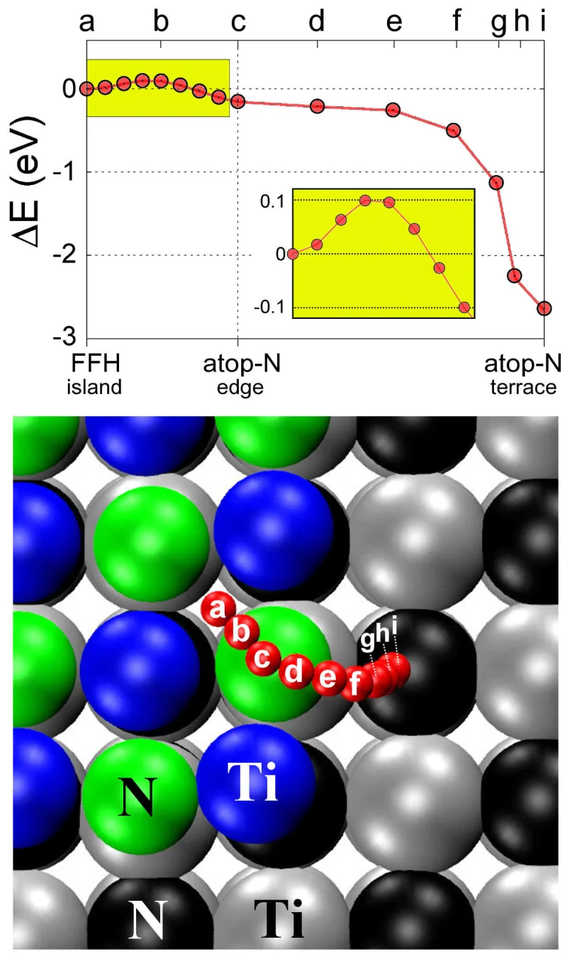
This tutorial builds upon the Ti Adatom on a 5×5 TiN Island tutorial, where the manuscript's 458-atom cell is created with the adatom at each site. The sites are labelled as in Fig. 6 of the manuscript: a, the fourfold hollow (FFH) on the island next to its edge; c, atop the N edge atom; i, atop the N terrace atom in front of the edge, the site that extends the island.

The figure below shows the descent path from the manuscript (Figure 6), the energies of states a to i above and the trajectory of the adatom below:

The manuscript calculates these energies with Density Functional Theory (DFT). This tutorial calculates them twice: with the MACE-MP-0 machine-learned force field in the notebook's own kernel, and with DFT on the Mat3ra platform, starting from the structures MACE relaxed. Section 4 lists the settings of both.

2. Prerequisites

The notebook loads four materials from the uploads folder by exact name and raises a KeyError when one is missing: TiN(001) 12x12x3 island 5x5, the island cell without the adatom, and the three cells with the adatom at a, c and i. All four are created and saved by defect_point_adatom_island_titanium_nitride.ipynb, the notebook of the Ti Adatom on a 5×5 TiN Island tutorial, which should be run first with the CELL_SIZE set in cell 1.2 here.

The MACE relaxations of Sections 2 to 6 run in the notebook's own kernel. The DFT relaxations of Section 7 are jobs on the Mat3ra platform and need an account on it.

3. Workflow overview

The adsorption energy at a follows Eq. (4) of the manuscript:

E_ads(a) = E(slab + island + Ti at a) − E(slab + island) − E_Ti

where E_Ti is the energy of an isolated Ti atom. The energies of c and i are taken relative to a, as on the vertical axis of Fig. 6. Both methods calculate the same four energies on the same structures. The steps are:

1. Set up the environment and parameters: install packages (JupyterLite only), material names, force field, relaxation, DFT and compute parameters
2. Load the materials: the island cell and the three adatom cells from the uploads folder
3. Build the MACE calculator: from the settings in cell 1.3
4. Relax the island cell: then measure the island contraction and the surface ripple
5. Relax the adatom at a, c and i: one relaxation per site, starting from the placed site
6. Calculate the energy of an isolated Ti atom: the reference of the adsorption energy
7. Run DFT on the platform: a fixed-cell relaxation on the four slab structures, each starting from the geometry MACE relaxed, and a total energy on the isolated Ti atom, which has nothing to relax
8. Compare with the manuscript: energies relative to a, the adsorption energy at a, and the Fig. 6 plot

4. Calculation parameters

4.1. Force field and relaxation

Cell 1.3 sets the force field and the relaxation; its DFT_MATERIAL_LABELS is in Section 5.4:

ORGANIZATION_NAME = None
FOLDER = "./uploads"

MACE_MODEL_FAMILY = "MACE-MP-0"
MACE_MODEL = "large"
MACE_DISPERSION = True
MACE_DEFAULT_DTYPE = "float64"
MACE_DEVICE = "cpu"

FMAX = 0.02  # eV/Å
MAX_STEPS = 1000
FROZEN_SLAB_PLANES = 1  # bottom slab planes held fixed in the MACE and DFT relaxations

Every MACE relaxation uses the Broyden–Fletcher–Goldfarb–Shanno (BFGS) optimizer of the Atomic Simulation Environment (ASE) and stops when the largest force falls below FMAX. FROZEN_SLAB_PLANES holds the atoms of that many bottom slab planes at their positions, in the MACE relaxations and in the DFT ones; every other atom is free. The notebook carries the fixed atoms into the DFT jobs as the material's atomic constraints, so both methods relax the same atoms. The isolated Ti atom is one Ti site at the centre of an otherwise empty cell the size of the island cell.

4.2. Cell size

CELL_SIZE in cell 1.2 names the cell the structure notebook built, and has to match the setting used there. The manuscript's cell, "12x12x3", has 457 atoms and 458 with the adatom; "10x10x2" has 225 and 226. Section 6 lists what each method gives on each of the two.

A DFT step on the manuscript's cell is several times the cost of one on the smaller cell, so the DFT jobs are run with CELL_SIZE = "10x10x2" set in both notebooks.

4.3. DFT model parameters

Cell 1.4 sets the model of every DFT job:

# manuscript: VASP, every structure relaxed with DFT; here the DFT relaxation starts from the MACE-relaxed structure
APPLICATION_NAME = "espresso"
RELAXATION_SEARCH_TERM = "fixed_cell_relaxation.json"
TOTAL_ENERGY_SEARCH_TERM = "total_energy.json"  # the isolated atom: one SCF, nothing to relax
RELAX_UNIT = "pw_relax"
SCF_UNIT = "pw_scf"
# manuscript: GGA of Perdew, Burke and Wang (PW91); for PW91 add "input_dft": "pw91" to DFT_SYSTEM_SETTINGS
FUNCTIONAL = "pbe"
PSEUDOPOTENTIAL_TYPE = "us"  # manuscript: PAW; ours GBRV ultrasoft
ECUTWFC = 40  # Ry; manuscript: 400 eV for the static calculations, Sec. II.B
ECUTRHO = 200  # Ry
DFT_KGRID = [1, 1, 1]  # manuscript: Γ only
DFT_SYSTEM_SETTINGS = {"smearing": "mv", "degauss": 0.01}  # Ry
MAXIMUM_IONIC_STEPS = 5  # per job, so that it ends within TIME_LIMIT
DAVIDSON_SUBSPACE_DIMENSION = 2  # half the default 4: less memory per process
DFT_CONTROL_SETTINGS = {"nstep": MAXIMUM_IONIC_STEPS}
# conv_thr 1e-4 Ry ≈ 1.4 meV on the total energy; local-TF mixing for a slab with vacuum
DFT_ELECTRONS_SETTINGS = {"conv_thr": 1e-4, "mixing_mode": "local-TF", "mixing_beta": 0.2,
                          "diago_david_ndim": DAVIDSON_SUBSPACE_DIMENSION}
DFT_SPIN_SETTINGS_BY_LABEL = {"isolated_adatom": {"nspin": 2, "tot_magnetization": 2}}  # two unpaired Ti d electrons

Quantum ESPRESSO runs a fixed-cell relaxation on the four slab structures, and a total energy on the isolated Ti atom, which has nothing to relax, with the PBE functional and the GBRV ultrasoft pseudopotentials the platform publishes, at 40 and 200 Ry, on the Γ point alone, with Marzari-Vanderbilt smearing of 0.01 Ry. MAXIMUM_IONIC_STEPS bounds the ionic steps of one job so that it ends inside its time limit, and Section 8 reads each structure at that step. conv_thr of 1e-4 Ry and local-TF mixing at 0.2 are what converge this metallic slab, and DAVIDSON_SUBSPACE_DIMENSION halves the Davidson subspace to lower the memory each process needs. Of the five structures only the isolated Ti atom is spin-polarized, at a fixed total magnetization.

4.4. Compute resources

Cell 1.5 sets where the jobs run:

from mat3ra.ide.compute import QueueName

CLUSTER_NAME = "001"
QUEUE_NAME = QueueName.OF
PPN = 60  # OF's maxPPN: the job is billed for the whole node
TIME_LIMIT = "08:00:00"
POLL_INTERVAL = 600  # seconds

CLUSTER_NAME selects the cluster whose hostname contains it. PPN is the maximum of the OF queue, so the job uses the whole node it is billed for. TIME_LIMIT bounds one job, and POLL_INTERVAL is how often Section 7.9 asks the platform whether the jobs have finished.

4.5. Methods compared with the manuscript

The manuscript uses DFT with the Generalized Gradient Approximation (GGA) in the Vienna Ab initio Simulation Package (VASP), and relaxes every structure with DFT at 0 K (Sec. II.A); its bottom slab layer is held fixed in the molecular dynamics runs. This tutorial relaxes every structure with the MACE-MP-0 large model with the D3 dispersion correction, in double precision (float64) on the CPU, and the DFT relaxation then starts from that geometry and takes the ionic steps MAXIMUM_IONIC_STEPS allows.

The site spacing here, from Standata's mp-492, is 2.121 Å against the manuscript's nearest-neighbour distance of 2.127 Å (Sec. II.A). The manuscript cites its isolated Ti atom energy (−2.275 eV); this tutorial calculates its own with each method. Sec. II.B of the manuscript pre-optimizes the atop-N-edge configuration (c) with the adatom's relaxation constrained along [001]; this notebook relaxes c with every atom but the fixed bottom plane free.

4.6. Dispersion and the browser

In JupyterLite, the install and calculator cells run, but the first relaxation exceeds the browser's memory: on the manuscript's cell, the first force call on its 457 atoms fails with can't allocate memory: you tried to allocate 763723776 bytes, a 0.76 GB tensor. The JupyterLite bundle also carries no torch-dftd, so D3 is off in the browser.

The four MACE relaxations, on the manuscript's cell of 457 and 458 atoms, run natively, with mace-torch and torch-dftd installed. The MACE values in Section 6 are from such a run. The DFT jobs of Section 7 run on the platform and do not depend on the kernel the notebook runs in.

5. Step-by-step instructions

5.1. Open the notebook

Navigate to the API examples repository and open the simulation notebook:

other/materials_designer/specific_examples/defect_point_adatom_island_titanium_nitride_SIMULATION.ipynb

5.2. Set the material names

Cell 1.2 names the materials the notebook loads:

# Names saved by defect_point_adatom_island_titanium_nitride.ipynb, with the CELL_SIZE set there.
CELL_SIZE = "12x12x3"
ISLAND_MATERIAL_NAME = f"TiN(001) {CELL_SIZE} island 5x5"
ADATOM_MATERIAL_NAMES = {
    "a": f"{ISLAND_MATERIAL_NAME} + Ti a (FFH island)",
    "c": f"{ISLAND_MATERIAL_NAME} + Ti c (atop-N edge)",
    "i": f"{ISLAND_MATERIAL_NAME} + Ti i (atop-N terrace)",
}

CELL_SIZE ships as the manuscript's cell, which Sections 2 to 6 relax with MACE. The DFT settings of cells 1.4 and 1.5 are sized for the smaller cell of Section 4.2: before running Section 7, set CELL_SIZE = "10x10x2" here and in the structure notebook, and run the structure notebook again so that the uploads folder holds that cell.

5.3. Run the MACE relaxations

Execute all cells by selecting Run > Run All Cells. Sections 2 to 6 need no platform account. The notebook:

1. Loads the four materials and prints their atom counts
2. Builds the MACE calculator
3. Relaxes the island cell and prints the island contraction and the ripple
4. Relaxes the adatom at a, c and i, and prints each energy and the adatom's displacement from its site
5. Calculates the energy of an isolated Ti atom

5.4. Run the DFT relaxations

DFT_MATERIAL_LABELS in cell 1.3 names the structures Section 7 runs, and ships empty, so Run All Cells submits nothing and Section 8 holds the MACE values alone:

# One platform job per structure: a fixed-cell relaxation on the MACE-relaxed slab structures, and a total
# energy on the isolated Ti atom, which has nothing to relax; an empty list skips the platform jobs.
# The structures can be added one at a time, each after the previous job has finished.
DFT_MATERIAL_LABELS = [
    # "slab_with_island",
    # "a",
    # "c",
    # "i",
    # "isolated_adatom",
]

Set CELL_SIZE = "10x10x2" as Section 5.2 describes before uncommenting any of them: Section 7 runs whatever cell the uploads folder holds, and on the manuscript's cell one job runs out of time before it reaches an energy. Uncommenting one label at a time, each after the job before it has finished, keeps one job on the cluster; a structure that already has a job is picked up again instead of being submitted twice.

Section 7 authenticates with the platform, initializes the API client, and selects the account and the default project whatever the list holds. With a structure listed, it then:

1. Saves the MACE-relaxed structures, each with the fixed bottom plane as its atomic constraints, and the isolated Ti atom
2. Builds the DFT model from cell 1.4
3. Creates the compute configuration from cell 1.5
4. Creates one job per structure and submits it — a fixed-cell relaxation, or a total energy for the isolated Ti atom — reusing a submitted, queued, active or finished job of the same workflow on the same structure
5. Waits for the jobs, polling every POLL_INTERVAL seconds
6. Reads the total energy of each job

5.5. Monitor progress

Each MACE relaxation prints one line per BFGS step: the step, the time, the energy, and the largest force. Each DFT job prints its identifier and its status when it is created, and the notebook then polls it until it finishes.

5.6. Read the results

Section 8.1 of the notebook prints this notebook's MACE and DFT values beside the manuscript's: the energies of c and i relative to a, the adsorption energy at a, the isolated Ti atom energy, the island contraction, and the ripple. A quantity whose DFT job has not run shows —. Section 8.2 plots the manuscript's states a to i of Fig. 6 (upper panel) as a line, with this notebook's a, c and i as markers on the same axes.

6. Expected results

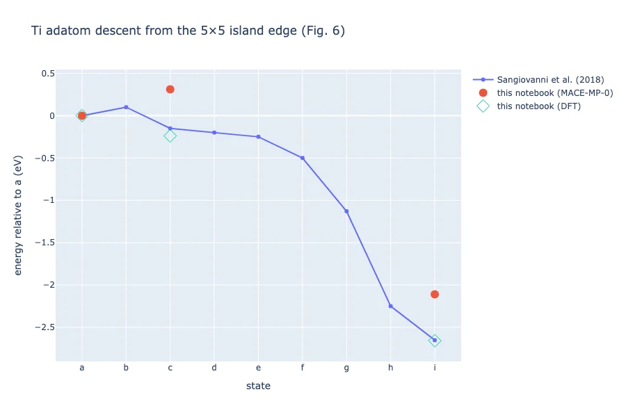
The table below holds every value this notebook computed, each beside the manuscript's and its source. The MACE columns are native runs on the two cells of Section 4.2; the DFT column is a fixed-cell relaxation of the four slab structures on the platform, started from the MACE geometry and read at its fifth ionic step, and a total energy on the isolated Ti atom, which has nothing to relax. At these settings DFT places c below a, as the manuscript reports, where MACE places it above.

Quantity	This notebook, MACE (12×12×3)	This notebook, MACE (10×10×2)	This notebook, DFT (10×10×2)	Sangiovanni et al. (2018)
E(c) − E(a), eV	0.315	0.311	−0.239	−0.15 ± 0.02 (Fig. 6, read off the axis)
E(i) − E(a), eV	−2.247	−2.109	−2.657	−2.65 ± 0.05 (Fig. 6, read off the axis)
E_ads(a), eV	−3.015	−3.067	−2.923	−2.81 (Sec. III.A ¶8)
E_Ti, isolated atom, eV	−3.889	−3.889	—	−2.275 (Sec. II.B)
Ti–Ti spacing along the island diagonals, % of bulk	−5.0	−5.1	—	−6.8 (Sec. III.A, p. 10)
Ti–N spacing along the island medians, % of bulk	−3.6	−3.7	—	−5.2 (Sec. III.A, p. 10)
Surface ripple, N above Ti, Å	0.071	0.028	—	0.19 (Sec. III.A, p. 8)

Quantum ESPRESSO's absolute energy for the free Ti atom is not on the manuscript's scale, so the DFT column leaves E_Ti out; it cancels in E_ads(a), where it is used.

The island contraction and the ripple are measured on the MACE relaxation only.

a: as built → MACE-relaxed (12×12×3)

MACE-relaxed a → c → i (12×12×3)

Section 8.2 of the notebook draws the manuscript's states a to i as a line, this notebook's MACE energies at a, c and i as filled markers, and its DFT energies at the same three sites as open diamonds, both on the 10×10×2 cell:

7. Customization options

7.1. Change the force field model

MACE_MODEL_FAMILY, MACE_MODEL, and MACE_DEFAULT_DTYPE in cell 1.3 select the model. Setting MACE_DISPERSION = False gives MACE without D3 in a native run as well.

7.2. Change the relaxation threshold

FMAX in cell 1.3 is the force threshold in eV/Å, and MAX_STEPS caps the number of BFGS steps of each relaxation.

7.3. Run more structures through DFT

Section 6's DFT column needs all five labels of DFT_MATERIAL_LABELS: slab_with_island, a, c, i and isolated_adatom. Each is uncommented after the job before it has finished, on the cell Section 5.2 sets.

8. Troubleshooting

8.1. Material not found

Section 2 of the notebook raises a KeyError naming the material when one of the four names in cell 1.2 is missing from the uploads folder. Re-run defect_point_adatom_island_titanium_nitride.ipynb, the notebook of the structure tutorial, in the same environment; it saves the four materials under the names in cell 1.2.

8.2. MACE is not installed

In JupyterLite, cell 1.1 installs MACE; it has to run before any other cell. Natively it installs nothing and prints To install packages, run `pip install ".[all]"` in the terminal; that extra does not include MACE. The native install is pip install ".[all]" mace-torch torch-dftd, followed by a kernel restart.

8.3. The run is without dispersion

When Section 3 of the notebook prints torch-dftd is not available here: MACE runs WITHOUT the D3 dispersion correction., every energy is MACE alone and differs from Section 6. This is the case in every JupyterLite run (Section 4.6). The values of Section 6 need a native kernel with torch-dftd installed.

8.4. The relaxations take long

Every BFGS step evaluates MACE on all the atoms of the cell, 457 or 458 on the manuscript's, and the notebook runs four relaxations; in JupyterLite the first one stops on the browser's memory limit (Section 4.6).

9. Interactive JupyterLite notebook

The following JupyterLite notebook relaxes the Ti adatom at a, c and i with MACE and with DFT, and compares the energies with the manuscript. In the browser, the install and calculator cells run and the relaxations do not (Section 4.6).

⛶ Full Screen

10. References

---

1. D. G. Sangiovanni, A. B. Mei, D. Edström, L. Hultman, V. Chirita, I. Petrov, and J. E. Greene. Effects of surface vibrations on interlayer mass transport: ab initio molecular dynamics investigation of ti adatom descent pathways and rates from tin/tin(001) islands. Physical Review B, 97:035406, 2018. URL: https://link.aps.org/doi/10.1103/PhysRevB.97.035406. ↩